My friend Marcus Mao (I'd call him "Chairman Mao") is working on his research program on this topic, and I was honorably invited to do the data analysis part of his work. The data came from testing the length of telomere of cells from human hair. Obtaining the data can be tough and time consuming, but let's keep it simple and just focus on the data analysis itself.
Package Preparation
Python is used to tackle the data analysis work in this article. Package used includes pandas (for constructing data frame), numpy (for calculation), sklearn (for calling linear model), and matplotlib (for plotting result). The statements to import these packages are listed.
1 | import pandas as pd |
Data Observation
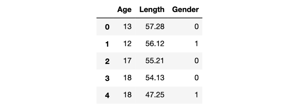
The data for this analysis task is provided by Chairman Mao (highest respect to him for spending days and nights in the biology lab). 29 samples are provided as a csv file. Each row contains the length of the telomere (Chairman Mao has taken the average during his work). Besides the length of the telomere, the age and gender of the participant are also recorded. The following subsections in this section aim to reveal the relationship between age and gender with the length of the telomere.
Before working on the data analysis problem, the data needs to be imported. The data import command is illustrated as follows. Note that the value of gender is represented with 0 and 1, which stand for male and female.
1 | telomere_df = pd.read_csv('./telomere.csv') |
Here's a glance of the data frame.
Data Distribution
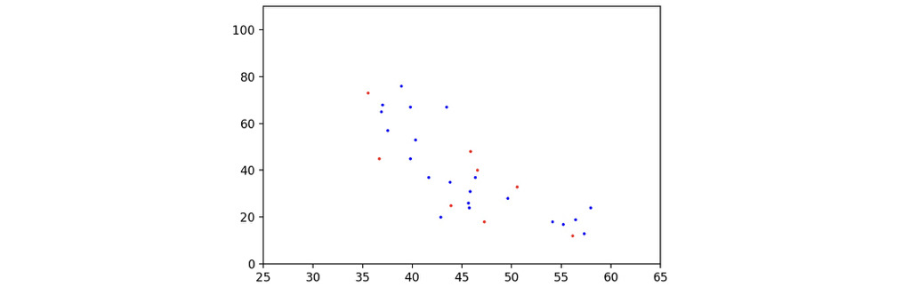
To illustrate the distribution of the sample data, I used matplotlib to draw the scatter map of the data. Gender is annotated by different colors: red is for females, and blue is for males. The x-axis represents the length of the telomere, and the y-axis represents the age of the corresponding participant. The following code would help to draw the scatter map.
1 | male_df = telomere_df[telomere_df['Gender'] == 0] |
Here is the scatter map of the data samples. As can be seen, they seem to have some relationships, instead of a bunch of random noise, not bad!
Correlation between Variables
The relationship between two distributions can be determined with correlation, usually represented as \(r\). The interval which \(r\) lies on is \([-1, 1]\), the greater absolute value it has, the stronger relationship there is between the two distributions. If \(r\) is positive, it means the two distributions are positively related, otherwise they are negatively related. Here is the formula to calculate the correlation between two random variables \(X\) and \(Y\). \[
\newcommand{\Cov}{\mathrm{Cov}}
\newcommand{\Var}{\mathrm{Var}}
r = \frac{\Cov(X, Y)}{\sqrt{\Var(X)}\sqrt{\Var(Y)}}
\] The correlation between variables can be obtained with corr method of the data frame, as follows.
1 | telomere_df.corr() |
The result of the code shows the correlation between length of telomere and age is \(-0.798634\), and the correlation between length of telomere and gender is \(-0.015549\). It is obvious that the length of telomere and age is negatively correlated, which corresponds to our biology knowledge, while there is almost no relationship between gender and the length of telomere.
Data Transformation
Since I only got 29 data samples, sophisticated regression models such as support vector regression or even multilayer perceptron should not be adopted. Linear regression seems to be a simple but good enough solution, but it has no non-linearity component. Luckily, the data transformation would help to release this problem a little, that is the box-cox transformation.
If you feel like getting to know the details of box-cox transformation, you can refer to another blog of mine, which includes the representation of the transformation as well as the Python implementation. By calling the function defined in the blog, it can be seen that the optimal \(\lambda\) selection is \(0.02020202\), which is close enough to 0. For the simplicity of the transformation, I just took \(\lambda = 0\), and the transformation is implemented as follows.
1 | telomere_df['Ln_Age'] = np.log(telomere_df['Age'].values) |
Modelling
After applying the box-cox transformation, I just need to use the following linear model to finish the regression task. Given the feature vector \(\textbf{x}\) and label \(y\), the linear model is illustrated as follows. \[
y = \Theta \textbf{x} + e
\] In which \(\Theta\) is the trainable parameter and \(e\) is the random noise that conforms to normal distribution. The best \(\Theta\) is obtained by minimizing the square error \(Q(\Theta)\) of the model over the training dataset. \[
Q(\Theta) = \Vert y - \Theta \textbf{x} \Vert ^2
\] sklearn.linear_model.LinearRegression was used to optimize the linear model, which saved lots of efforts. The implementation is just two lines of code.
1 | regressor = linear_model.LinearRegression() |
By calling the attribute coef_ and intercept_of sklearn.linear_model.LinearRegression, we can obtain the coefficients of our linear model.
1 | print(regressor.coef_) |
With consideration of the box-cox transformation, I can give the following prediction formula of the predicting problem, in which \(l\) stand for the length of telomere and \(g\) stand for gender. \[ \newcommand{\euler}{e} y = \euler^{6.55718 -0.06627l - 0.08695g} \]
Result
In this section, I would summarize the findings, as well as run some tests to judge whether the model is good enough for prediction.
\(R^2\) Statistics of Model
There are multiple ways for judging the performance of a regression model, including mean square error and \(R^2\) statistics. The latter statistics, say, \(R^2\) statistics, could represent how good is the regression model, in brief, \(R^2 = 1\) means the model perfectly fit the test data without error, while \(R^2 = 0\) means that the model is not better than predicting the label with the mean of label that you observed. (If \(R^2 < 0\), it means that the model is so ridiculous that it is even worse than predicting everything with observed average value!) The \(R^2\) statistics of the model can be obtained with the following code.
1 | print(regressor.score(telomere_df[['Length', 'Gender']].values, telomere_df['Ln_Age'])) |
The \(R^2\) of the model is \(0.69728\), which is not a bad score, I'd say, and Chairman Mao's research project finally got a good result 😊. If the model is trained without box-cox transformation (just replace the indices Ln_Age with Age), the \(R^2\) is \(0.6431685\), proving that box-cox transformation does help to fine-tune the model.
Prediction Plotting
To predict the label list with a given feature list, we can call predict method of the regressor, implemented as follows. Do not forget to apply the exponential transformation of the result since the label obtained directly from the linear model is the natural logarithm of age.
1 | np.exp(regressor.predict(feature_list)) |
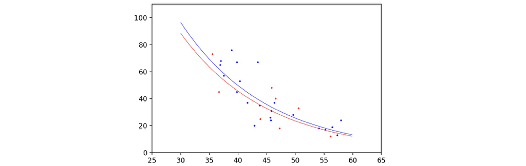
The following command would help to plot the curve of our prediction along with the scatter points of our samples. Since the two dimensional feature cannot be represented with only one axis, I plotted two curves, assuming gender is male or female, and the length of telomere varies with axises.
1 | male_axis = np.array([np.array([axis, 0]) for axis in np.arange(30, 60, 0.1)]) |
The plot is as follows, although the gender does cause a difference, the two curves look basically the same, looks good enough!